You are handed a brain MRI and a deceptively simple question: how much multiple sclerosis is in here? The lesions are right there on the FLAIR scan, bright little blobs scattered through the white matter, but “right there” is not a number. Counting them by hand across 181 slices, for five patients, is how you lose a weekend. This post walks through an unsupervised pipeline that turns those blobs into a single value: lesion load in cubic millimeters.
TL;DR: Build an unsupervised pipeline that segments multiple sclerosis lesions in brain MRI and reports lesion load in cubic millimeters.
Stack: Python, SimpleITK, ITK-Elastix, scikit-learn, NumPy
Level: Advanced
Reading time: ~6 min
I built this for a 3D image processing course, with five patient scans, a probabilistic brain atlas, and a grading rubric that handed out a flat zero if the notebook threw a single error. No ground truth labels, no shortcuts. Just raw T1 and FLAIR volumes and the expectation that, by the end, a spreadsheet of lesion volumes would fall out the other side.
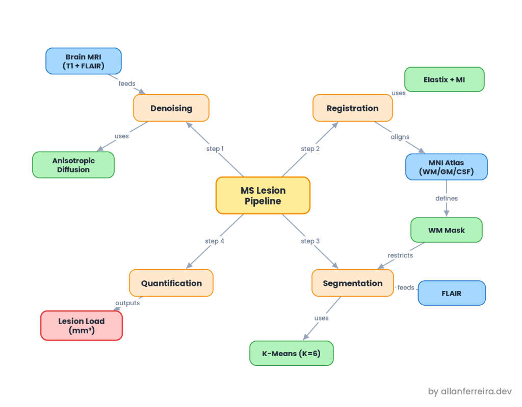
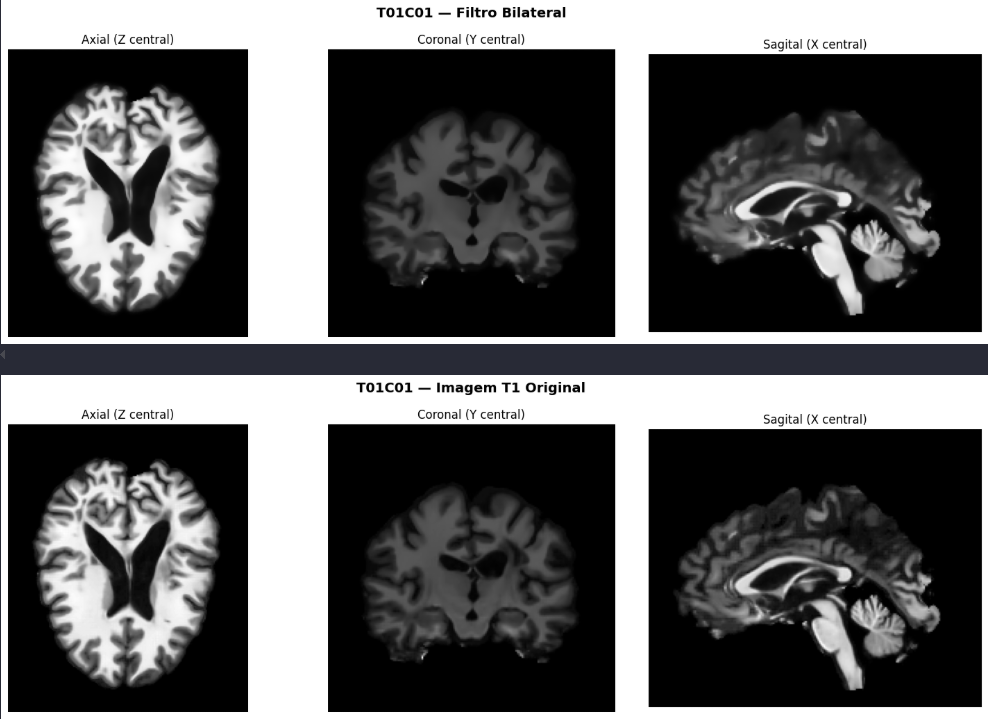
Kill the noise before anything else
MRI does not arrive clean. The scanner, the patient breathing, heat in the coils, all of it leaves noise that later steps will happily mistake for signal. The catch is a tradeoff: filter too little and the noise survives, filter too much and you erase the fine edges that matter for diagnosis. So I tested three denoisers and let a difference image referee them.
The judge is simple. Subtract the filtered image from the original and look at what got removed:
G = np.abs(arr_original - arr_denoised)
If G is just random grain, the filter took out noise and nothing else. If G shows crisp brain anatomy, the filter went too far and deleted real structure. Bilateral smoothed too aggressively. Non-Local Means looked great in theory but never finished on a full volume in reasonable time, so it was out on cost alone. Anisotropic diffusion won: it smooths hard inside flat regions and nearly stops at edges.
f = sitk.GradientAnisotropicDiffusionImageFilter()
f.SetNumberOfIterations(10)
f.SetConductanceParameter(1.0)
f.SetTimeStep(0.0625)
img_denoised = f.Execute(sitk.Cast(img, sitk.sitkFloat32))
I backed the visual call with SSIM (0.998, structure preserved), so the choice was not pure eyeballing.
Get the atlas and the patient into the same space
Here is the core problem. The probabilistic atlas (maps telling you, per voxel, the chance of white matter, gray matter, or CSF) lives in a standard coordinate space. The patient’s brain does not: different position, different size, different shape. To use the atlas as a guide, you first have to warp it onto the patient, and that takes registration.
Those maps live in MNI space, named after the Montreal Neurological Institute, which built the template by averaging hundreds of healthy brains into one canonical head. That averaging is exactly why you cannot compare intensities directly: the atlas brightness is a blend of many people, not this patient.
So the similarity metric is Mutual Information, which scores statistical consistency between intensity distributions instead of raw pixel difference. The registration runs in two passes, coarse to fine:
parameter_object.AddParameterMap(rigid_params)   # global position and rotation
parameter_object.AddParameterMap(affine_params)  # scale and shear

result, transform = itk.elastix_registration_method(
    fixed_image, moving_image, parameter_object=parameter_object)
Whatever transform aligns the atlas T1 gets applied identically to the WM, GM, and CSF maps, with linear interpolation so their 0 to 1 probabilities stay smooth. To check the result without ground truth, I used a checkerboard: interleave blocks of both images and see if the anatomy flows across the seams. It did.
Find the bright outliers in the white matter
MS is a white matter disease, and on FLAIR the lesions are hyperintense, brighter than the tissue around them. That hands you a strategy: look only inside white matter, then hunt for the brightest cluster.
The atlas builds the mask. A voxel counts as white matter only if the maps agree strongly:
mask = (wm > 0.8) & (gm < 0.3) & (csf < 0.2)
The two negative conditions matter more than they look. They cut voxels near the cortex and the ventricles, where partial volume effects fake brightness, and periventricular tissue is exactly where many MS lesions hide.
Then K-Means on the FLAIR intensities inside that mask, with K=6. Why not K=2, lesion versus normal? Because normal white matter already varies in brightness, so a two way split would shove every slightly bright voxel into the lesion group and inflate the count. With six clusters, the natural variation spreads across five “normal” buckets and the brightest one isolates the hyperintense tail. That cluster, refined by an adaptive intensity threshold and cleaned of blobs smaller than 3 voxels, is the lesion.
Turn voxels into millimeters
The last step is almost anticlimactic. Count the lesion voxels and multiply by the volume of one voxel:
volume_mm3 = np.count_nonzero(lesion_mask) * np.prod(spacing)
The scans are 1 mm isotropic, so each voxel is exactly one cubic millimeter and the count is the volume. Five patients, five numbers:
| Image | Lesion load (mm³) |
|---|---|
| T01C01 | 14101 |
| T01C04 | 25474 |
| T03C04 | 6247 |
| T04C03 | 16239 |
| T05C02 | 7927 |
The detected lesions clustered around the ventricles, the periventricular pattern the McDonald criteria flag as typical for MS. Not proof, but a reassuring sign that the pipeline found disease and not artifacts.
What you have done
You took raw T1 and FLAIR volumes, stripped the noise with anisotropic diffusion, warped a probabilistic atlas onto each patient with a rigid then affine registration, masked down to confident white matter, and let K-Means surface the hyperintense lesions. Then you counted voxels and got a real clinical number, lesion load in cubic millimeters, with no manual tracing and no labeled training data. The weekend is yours again.
Next steps
- Add N4 bias correction: Run N4 right after denoising to flatten the slow intensity drift the coils introduce. It makes the white matter threshold far more stable across patients.
- Swap K-Means for a GMM: A Gaussian Mixture gives soft, probabilistic cluster membership instead of hard labels, which handles the fuzzy lesion boundary better.
- Validate against a radiologist: Compare the volumes to expert manual segmentations with a Dice score, turning “looks right” into a measured error.
- Try deformable registration: A B-spline pass after the affine step would close the cortical mismatch that the rigid plus affine cascade leaves behind.
Questions or feedback? Find me on LinkedIn or GitHub.