Somebody opens a photo in Photoshop, erase a tiny scratch in the background, save, and post it online thinking nobody will notice, and nobody notices, looking at it with the eye. Except the camera noise noticed, and it is going to tell. This post is about how a classical signal-processing technique, with zero lines of deep learning, can point at exactly where the image was tampered with.
TL;DR: How a Python POC detects photo edits using only statistical analysis of the sensor’s gaussian noise, with no trained model, no AI, and no GPU. Trade-offs and limits included.
Stack: Python, NumPy, SciPy, PIL, signal processing
Level: Intermediate
Reading time: ~6 min
Every time someone edits a photo, they leave a trace. Professional forensic tools have known this for decades. But most of the current conversation about tampered-image detection revolves around deep learning models trained on huge datasets, with compute cost to match. It works, but it covers a problem that statistics handles in most cases without going anywhere near a GPU.
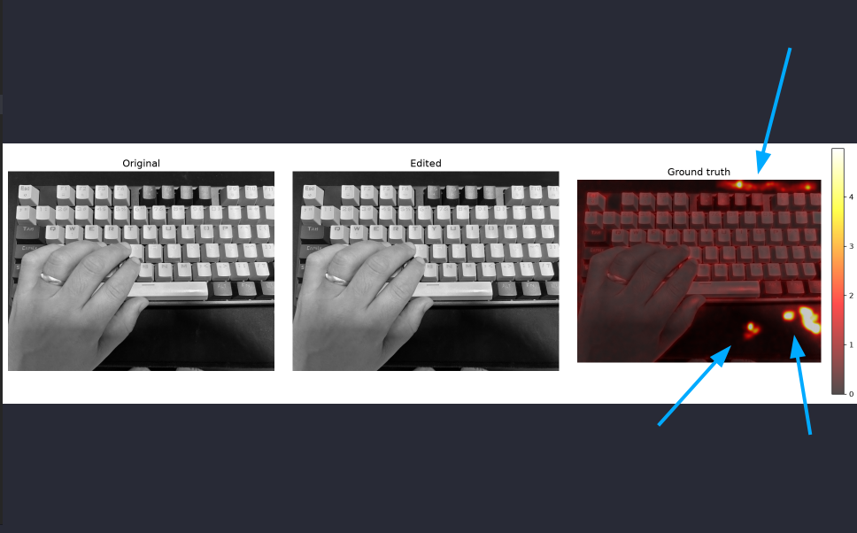
I spent an afternoon playing with a photo of my keyboard. I edited out some tiny scratches on the desk pad, the kind nobody would ever spot. Then I opened Python to see if I could rat myself out, without giving the algorithm access to the original file. It worked in two hours of code, and I did not train anything.
Why your camera noise gives you away
A CCD or CMOS sensor is not perfect. Every photo it takes picks up a random noise pattern, invisible to the naked eye, that follows a gaussian distribution with a sigma specific to the camera, the lighting of the scene, and how hard the JPEG squeezed it. Two photos taken by the same camera in the same light will have similar noise signatures. A region pasted from somewhere else (Photoshop brushing, AI generation, another photo altogether) brings a different signature, and there is no way to hide it.
Isolating the noise with a simple trick
A gaussian blur estimates the “clean content” of the image, meaning edges, shapes, and contrast. If you subtract the smoothed version from the original, what is left is exactly what oscillated at high frequency. That is the noise.
def noise_residual(image, sigma):
    smooth = gaussian_filter(image, sigma=sigma)
    return image - smooth
Three lines. None of them new. Signal processing has been doing this kind of decomposition since before my father was born. The novelty is not in the technique, it is in using it for a problem where a lot of people today would skip straight to a neural network.
Computing local standard deviation without a Python loop
The next step is to sweep the image in windows of 32 by 32 pixels and compute the standard deviation of the noise inside each window. Writing that as a pure Python loop takes hours on a large image. It does not have to. The variance identity handles it:
Var(X) = E[X²] − (E[X])²
def local_std(image, window):
    mean = uniform_filter(image, size=window)
    mean_sq = uniform_filter(image ** 2, size=window)
    variance = np.clip(mean_sq - mean ** 2, 0, None)
    return np.sqrt(variance)
Two passes of a moving average, one subtraction, one square root. Everything vectorized through SciPy. It runs in milliseconds on a 1000 by 1000 image.
The window size is the only delicate trade-off in this step. A small window (16 by 16) gives noisy statistics and lots of false positives. A large window (64 by 64) loses spatial resolution and the final heatmap smears. I landed on 32 by 32 by feel, the kind of feel that only shows up after running dozens of similar analyses before (thank you, PhD in computer vision).
Comparing each window against the global mean
With the local standard deviation in hand, each window gets a score that says how far it sits from the global mean of the noise, measured in “sigmas of distance”:
def anomaly_map(std_map, smooth_sigma):
    global_mean = std_map.mean()
    global_std = std_map.std()
    raw = np.abs(std_map - global_mean) / (global_std + 1e-9)
    return gaussian_filter(raw, sigma=smooth_sigma)
Regions above two sigmas are statistical anomalies, meaning noise that does not belong to the main distribution of the photo. A final blur on the heatmap smooths isolated pixels that show up by chance and highlights coherent regions that show up because the image was tampered with there.
The result
Looking at the comparison, the first three panels show the original photo, the edited one, and the ground truth (the direct difference between the two, which only exists because I had both images in hand). It serves as a reference. What actually matters is the fourth panel, the gaussian analysis running on its own, without access to the original, and calling out exactly the regions I edited.
The insight that matters here
When you need to detect something, the first instinct today is “I will train a model.” This is wrong more often than most people admit. Before training, always ask: is there a statistical or mathematical property that already gives away what I want to detect? If there is, it costs zero compute, runs anywhere, and you keep control of what you are doing. A model is a black box that does something else when you are not looking. An equation is always the same thing.
This connects directly with what I wrote about MIDAS. The choice between a proprietary model, an open VLM, or a frontier API is the same choice at another level: what is the cheapest tool that clears my quality bar? Here the bar cleared with three ten-line functions.
Where this technique fails (and it will fail)
I will be honest about the limits, because a technical post that only tells you what worked is marketing.
It does not work well on images that have been JPEG-compressed twice, because the second JPEG homogenizes the noise. It does not catch very small edits (a few dozen pixels), because the 32-pixel window does not really enclose the tampered region. It does not detect global transformations like changing brightness, contrast, or saturation on the whole image, because the noise stays consistent everywhere. And it fails on photos with heavy intentional grain (high ISO, analog filters), because the natural noise is already large and the signature of the pasted region drowns in it.
Each of these limits has a technique that covers it. PRNU analysis for sensor-specific signatures. DCT coefficient analysis to catch recompression. Combining multiple statistical estimators for robustness. But that is another post.