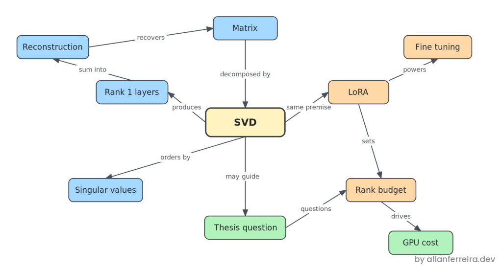
You kick off a fine-tuning run on a foundation model, watch the GPU meter climb, and pay for every second of it. Somewhere in that run, a decent chunk of compute is going into layers that have nothing to do with your problem. You do not know which ones, because nobody ever told you to ask. This post is about a way to start asking, and it begins somewhere unexpected: a photo of a tree in the snow.
TL;DR: How SVD decomposes a matrix into layers ordered by importance, why that is the same premise behind LoRA, and what it might mean for choosing where to spend a fine-tuning budget.
Stack: Python, NumPy, Pillow, SVD, LoRA
Level: Intermediate
Reading time: ~7 min
The problem underneath is that information does not spread evenly, but our adaptation budget usually does. When you attach LoRA adapters to a model, the common practice is to pick a rank and apply it uniformly across the layers you decided to touch, as if every one of them held the same amount of what your domain needs. In convolutional networks the old intuition at least gave you a starting point, since early layers learn generic edges and textures while later ones specialize, a pattern Yosinski and colleagues measured back in 2014. Transformers blurred that map. Attention and feed forward blocks do not sort themselves into generic and specific in any tidy way, so the honest answer to “which layers matter for my task” is that most of us are guessing, and paying GPU hours for the guess.
My advisor handed me this problem sideways. He told me to go study SVD, said the thesis would revolve around it, and left me to figure out why. So I did what I usually do when a concept refuses to become concrete: I wrote the smallest possible script that would let me see it. Grayscale photo in, decomposition out, one image per layer. Two hundred lines later the abstraction had a face.
A matrix is a stack of layers
Singular Value Decomposition takes any matrix and factors it into three pieces, W = U Σ Vᵀ. What matters here is not the algebra but what falls out of it: you can rewrite that product as a sum of very simple matrices, each one built from a single column of U, a single row of Vᵀ, and a scalar weight from Σ.
def monta_camada(matriz_U, pesos, matriz_Vt, numero_camada):
    indice = numero_camada - 1
    coluna = matriz_U[:, indice]
    linha  = matriz_Vt[indice]
    peso   = pesos[indice]
    return peso * np.outer(coluna, linha)
Each of those is a rank one matrix, the simplest non trivial thing a matrix can be. Stack them all and you get the original back, exactly. Stack only the first few and you get an approximation. The useful part is the ordering: the weights in Σ come out sorted from largest to smallest, so layer one carries more of the matrix than layer two, which carries more than layer three, all the way down to a long tail of layers that carry almost nothing.
Running it on a photo
Grayscale images are convenient here because a photo already is a matrix, one number per pixel. I ran the decomposition on a 336 by 296 shot of a lone tree in the snow, which is 99,456 numbers in total, and then reconstructed it from the first 35 layers out of the 296 available.
imagem:            336 x 296  (99,456 numeros)
camadas geradas:   35 de 296
reconstrucao:      22,155 numeros (22.3% do original)
imagem capturada:  99.8%
Twenty two percent of the numbers, ninety nine point eight percent of the information. Side by side with the original, the reconstruction loses some fine grain in the snow texture and holds everything else: the tree, the shadow, the horizon, the light. The storage math is easy to check, since keeping k layers means keeping k columns of U, k rows of Vᵀ and k weights, so 35 times (336 + 296 + 1) lands exactly on those 22,155 numbers.
Looking at the individual layers is what made it click for me. On their own they look like nothing, just gray fields with faint interference patterns, because a rank one matrix has no business resembling a photograph. The first ones carry broad structure, wide bands of light and dark. By layer fifteen they are fine texture. By layer thirty they are close to noise. None of them is the image, and all of them together are.
There is a nice historical wrinkle here. SVD itself goes back to Beltrami in 1873, but the guarantee that truncating it gives you the best possible approximation at that rank only arrived in 1936, when Eckart and Young proved it. Sixty years of people using a tool without knowing it was optimal.
Summing the layers back
The claim that the image is the sum of its layers is easy to state and easy to doubt, so it is worth proving. A second script loads the saved layers and adds them, nothing else.
def soma_das_camadas(arquivos_de_camada):
    acumulador = None
    for caminho in arquivos_de_camada:
        camada = np.load(caminho)
        if acumulador is None:
            acumulador = np.zeros_like(camada)
        acumulador += camada
    return acumulador
No weighting step in there, and that trips people up on first read. The weight is already baked into each saved layer, applied back when it was built with peso * np.outer(coluna, linha). One detail worth flagging: the sum has to run over the raw arrays, not the PNGs. The PNGs were re centered around mid gray so that negative values would be visible, which is fine for looking and useless for adding.
Where LoRA comes in
If the previous section felt like a linear algebra exercise, this is where it stops being one. LoRA, the most widely used fine tuning technique today, rests on exactly this premise. Instead of updating a weight matrix W directly, it freezes W and learns an update ΔW = BA, where B and A are skinny matrices whose product has low rank. The bet Hu and colleagues made in 2021 was that the change a model needs in order to adapt to a new task has low intrinsic rank, which in the language of this post means it fits in the first few layers of the stack.
That bet paid off, and spectacularly. But notice what it settles and what it leaves open. It settles that the update is low rank. It says nothing about whether the rank budget should be the same for every weight matrix in the model, which is the part everyone quietly assumes.
The question I am chasing
Here is the hypothesis my thesis is built on. If information concentrates unevenly inside a single matrix, and the photo makes that hard to argue with, then it should also concentrate unevenly across the layers of a trained model. Some layers of a foundation model should hold much more of what a specific domain needs than others, and the decomposition should be able to tell us which. The follow up question is what to do about it, because depending on the scenario it may make more sense to touch the structure than the weights.
I am not the first person in this neighborhood. AdaLoRA, from Zhang and colleagues in 2023, already allocates rank budget adaptively across weight matrices using an SVD style parameterization and an importance score, and any honest version of this idea has to start by reading that work carefully. Where I want to push is upstream of the allocation: not just how much budget each matrix gets during training, but whether the decomposition can say something about domain fit before you spend anything.
If it holds, the payoff is unglamorous and practical. Fewer trained parameters, fewer GPU hours, same result. In a year where hyperscaler capex is crossing a trillion dollars and an MIT study found that ninety five percent of companies investing in AI saw no return, unglamorous and practical is having a moment.
It may not hold. That is what the next few years are for.
What you have done
You watched a photograph get taken apart into 296 layers ordered by importance, saw the first 35 of them carry almost all of the image, and then put them back together by plain addition. Along the way the same idea turned out to be the foundation of the most common fine tuning technique in use today, which is a decent return on a two hundred line script and an afternoon.
Next steps
- Run it on your own images: Try a photo with dense texture, a crowd or foliage, and watch how many more layers you need for the same fidelity. Low complexity scenes like snow flatter the technique.
- Plot the singular values: The decay curve tells you more than any single reconstruction. A steep drop means the matrix is compressible, a flat one means it is not.
- Read the LoRA paper, then AdaLoRA: In that order. The first sets up the low rank premise, the second is the beginning of the argument about where the budget should go.
- Look at your own fine tuning config: If you are applying the same rank everywhere, that is a guess. It may be a good guess, but it is worth knowing that it is one.
Questions or feedback? Find me on LinkedIn or GitHub. The POC code is at github.com/ferrerallan/poc-svd.